What COVID did to our forecasting models (and what we built to handle the next shock)

How Airbnb built forecasting models resilient enough to survive a global pandemic and whatever shock comes next.

By: Harrison Katz

The week everything broke

In March 2020, the forecasting models that had served us well in stable times faced a new challenge: predicting outcomes in a world that had suddenly changed.

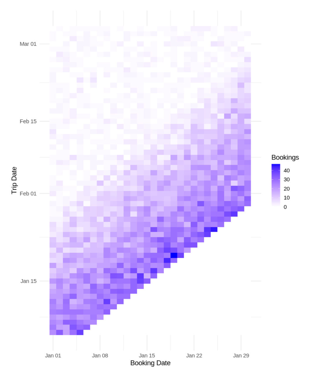
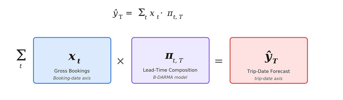
At Airbnb, many of the financial metrics we forecast depend on two separate events: when guests book, and when they actually travel. A booking made today might correspond to a trip three days from now or three months from now. The distribution of that gap, what we call the lead-time composition, drives how we translate today’s bookings into future revenue (see Figure 1).

The pandemic reshaped what was being booked and where. Hosts shifted their inventory toward longer stays and remote-friendly properties, while guests pivoted from urban centers to rural and suburban destinations. These supply and demand shifts interacted with each other over time, as hosts adapted listings to match evolving guest preferences and new inventory attracted new traveler segments.

Each of these dynamics introduces its own forecasting challenges, but they fall outside the scope of this article. Here, we focus on a more fundamental structural problem: the disruption of the lead time relationship between booking and travel.

Our models had learned stable patterns from years of data: seasonal rhythms, day-of-week effects, gradual trends. Then, as COVID took hold, lockdowns hit. A reopening would trigger a surge of demand, which would then reverse a week later. Rolling closures across different regions created patterns no historical data could have anticipated.

This is not a story unique to Airbnb. Every forecasting team at every company that deals with time-shifted metrics, such as insurance claims, subscription renewals, and supply chain orders, faced a version of the same problem. The specific challenge we want to highlight here is not just that the numbers changed. It’s that the structure of the data changed, and our models were not designed to detect or adapt to structural shifts.

This post describes what we observed, the architectural decision it forced us into, and the second surprise we discovered once the dust settled.

The architectural insight: separate the what from the when

Before COVID, we forecasted trip-date metrics more or less directly. The models learned the relationship between bookings and eventual trips as an integrated process. This worked when the relationship was stable. During the pandemic, it stopped working because two things were moving at once: the volume of bookings, and the temporal distribution of when those bookings would be realized as trips. A third variable shifted as well: whether bookings would be realized at all. Cancellation rates spiked and became far less predictable, adding another layer of instability to the booking-to-trip relationship. That problem deserves its own treatment and is not the focus here, but it compounds everything that follows.

The lockdown-reopening-relockdown cycle was the forcing function. Different regions would go into lockdown, reopen at different times, then often, and unpredictably, go back into lockdown again.

Gross booking volumes were swinging wildly as restrictions changed, but so was the lead-time composition. When a region reopened, people would book trips for the subsequent week. When a new variant hit, last-minute bookings dried up, but far-out bookings for “someday, when this is over” persisted.

The two signals were tangled together, and models that tried to learn them jointly could not disentangle which changes were driven by surges in volume and which were structural shifts in booking behavior. This led us to a fundamental architectural decision: decompose the forecast into two separate components:

1. Gross metrics on the booking date axis. How many bookings (nights, fees) are we recording each day? This is a standard univariate (or multivariate) time series problem.
2. Lead-time composition. Of the bookings recorded today, what fraction correspond to trips happening in each future time window? This is a compositional time series, a vector of proportions which must sum to one. The final trip-date forecast is the product of the two: gross bookings, multiplied by the lead-time composition vector, so the booking-date axis generates the trip-date axis.

This decomposition might sound obvious in hindsight, but it required a modeling framework that could handle compositional data natively. Standard time series methods do not respect the simplex constraint: that is, proportions must be non-negative and sum to one. Naive approaches such as forecasting each lead-time bucket independently produce incoherent results: the shares do not add up, and individual components can go negative.

We developed a family of models called B-DARMA (Bayesian Dirichlet Auto-Regressive Moving Average) specifically for this class of problem. The name unpacks the approach: the Dirichlet distribution enforces valid compositions, the auto-regressive and moving average components capture temporal dynamics in how those compositions evolve, and the Bayesian framework provides full predictive distributions with calibrated uncertainty while allowing us to encode domain knowledge through priors. The core model treats the lead-time composition as Dirichlet-distributed, with the mean vector evolving through a vector autoregressive process in log-ratio space. It learns temporal dependencies between the proportions and produces honest uncertainty bands, not just point forecasts.

We published the original methodology in the International Journal of Forecasting (B-DARMA; Katz, Brusch, & Weiss, 2024), and we have since extended the framework with variants for time-varying volatility (B-DARCH; Katz & Weiss, International Journal of Forecasting 2026), shrinkage priors for high-dimensional compositions, and the structural break intervention mechanism described below.

The two-part architecture (Figure 2) gave us something critical: the ability to diagnose which component was responsible when forecasts went wrong. During the lockdown cycle, gross volumes were volatile, but at least moved in interpretable ways (correlated with restriction announcements, case counts, and vaccination rates). The lead-time composition was the harder problem, and separating it out let us focus our modeling effort where the instability actually lived.

The second surprise: the distributions did not snap back

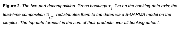
Here is where the story gets more interesting. By late 2021, gross booking volumes had largely recovered. You could look at top-line booking counts and conclude that things were back to normal. But when we looked at the lead-time compositions, the picture was different. The distributions had shifted during the pandemic and stayed shifted (Figure 3).

To quantify this, we started measuring the full distributional divergence between the current lead-time composition and a pre-pandemic baseline using a normalized L1 (Manhattan) distance. Instead of reducing the distribution to a mean or median, this captures the entire shape change: which parts of the distribution shifted, by how much, and whether they recovered. When we applied this approach to booking data across four major U.S. cities from 2018 to 2022, we found a clear two-phase pattern: an abrupt disruption at the pandemic’s onset, followed by a partial recovery that plateaued well short of pre-pandemic norms. The distribution did not return to its old shape; it settled into a new one (Figure 4). The divergence was especially pronounced for international guests, whose booking horizons compressed more sharply and recovered more slowly than domestic travelers. This is consistent with the layered effect of travel restrictions, visa uncertainty, and longer planning cycles that characterize cross-border travel. Even by late 2022, international lead-time distributions remained further from their pre-pandemic baseline than domestic ones.

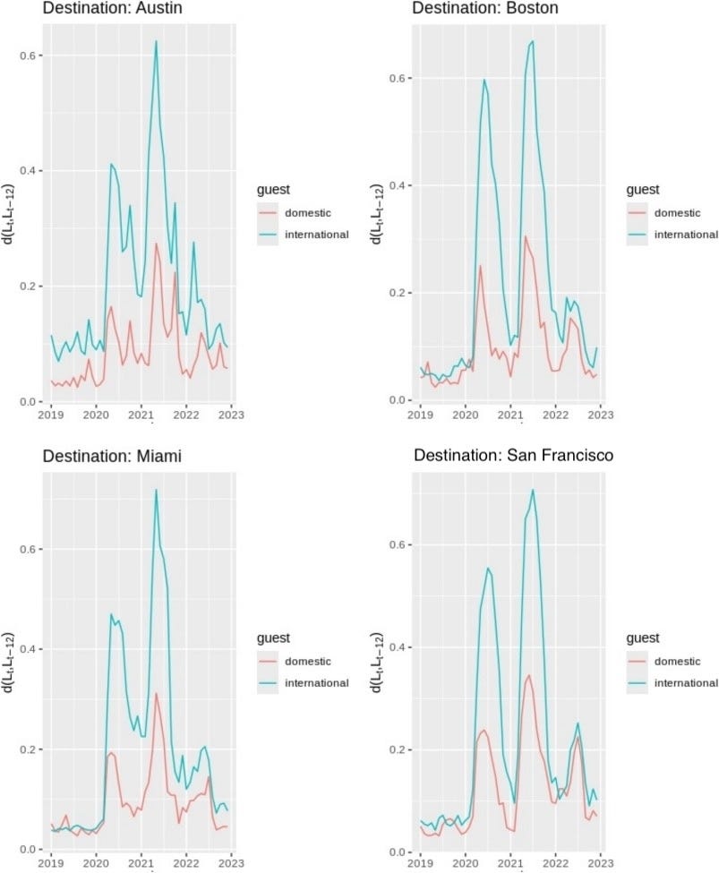
We published this analysis in Annals of Tourism Research: Empirical Insights (Katz, Savage, & Coles, 2025). We found similar persistence in stay-length distributions: the share of stays lasting 28 nights or longer nearly doubled during the pandemic, and remains significantly above its 2019 baseline, many years later.

This kind of monitoring turned out to be useful well beyond detecting exogenous shocks. The same distributional divergence metric that flagged the pandemic shift also became a diagnostic tool for model health. If the predicted lead-time composition is consistently diverging from the realized composition, that’s a signal that the model is misspecified, not just that the world changed. It lets us separate two failure modes that are easy to conflate: “the model is right but the inputs are unusual” versus “the model’s assumptions no longer hold,” even if the inputs were to revert toward previous norms.

Monitoring also gives us a measure of forecast stability over time. A model whose predicted distributions of lead times, cancellation rates, or regional booking shares are drifting gradually, even if point forecast accuracy looks fine, is a model heading toward a cliff. Catching that drift early, before it shows up in top-line error metrics, is where the real operational value is.

This was the second insight: even after the acute crisis passed, the compositional structure of our data had undergone a durable change. A model that assumed that pre-pandemic dynamics would eventually reassert themselves was going to produce systematically biased forecasts indefinitely.

Why distributional shifts hit the bottom line

These compositional changes were not just a statistical curiosity. At Airbnb, lead-time distributions feed directly into revenue forecasting, cash flow planning, and capacity decisions. The time gap between when a booking is made and when the guest travels determines when revenue is recognized, when cancellation risk resolves, and how far ahead operations teams can see incoming demand. When the composition shifts, every one of those downstream processes inherits the error. Getting the distributions right was a prerequisite for accurate financial operations.

Building models that learn structural shifts

The discovery of persistent distributional shifts, even as gross metrics stabilized, meant we needed B-DARMA to handle structural breaks natively rather than treating them as temporary anomalies to be dummied out. (“Dummying out” means adding a binary indicator variable, often called a dummy variable, that flags an unusual period so the model can ignore it rather than learn from it.)

We tried the obvious fix first: adding dummy variables for the COVID period. This worked in-sample (the model fit its training data well) but failed out-of-sample (it could not forecast new data accurately), and the reason is instructive. The pandemic was not a single fixed effect. It was a rolling sequence of distinct shocks: initial lockdowns, partial reopenings, the Delta variant, and the Omicron variant, each with its own directional impact on the lead-time composition. Fitting a separate dummy for each disruption period means estimating a new parameter every time the world changes, with no ability to generalize across shocks or project the trajectory forward. You end up with a model that perfectly explains the past and has nothing to say about the future.

What we needed was a model that could learn the direction and speed of a structural shift, not just flag that one has occurred. We extended B-DARMA with a directional-shift intervention mechanism that decomposes a structural break into three interpretable components:

1. A direction vector specifying which components of the composition gain share and which lose share during the transition.
2. An amplitude parameter controlling how large the redistribution is.
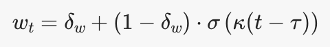
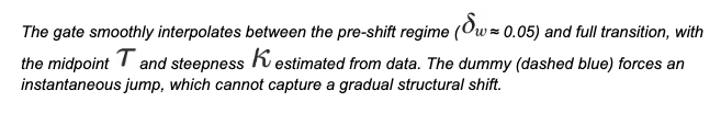
3. A logistic gate function governing the timing and speed of the transition, allowing for shifts over time rather than instantaneous jumps.

The logistic gate is the key. Instead of a binary before/after indicator, it learns a smooth S-shaped curve that ramps from 0 to 1 over a window of time. This means the model can represent both sudden shocks (steep curve) and gradual structural transitions (gentle slope), and crucially, it can project the transition forward into periods it has not yet observed (Figure 5).

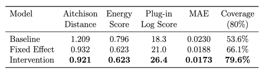
We tested this against the baseline B-DARMA and the dummy-variable approach using a rolling one-step-ahead forecast evaluation during peak COVID disruption (July 2020 through March 2021). The evaluation window begins in July because the intervention model requires several months of post-shock observations to estimate the new regime’s dynamics. In practice, this also reflected the reality of the moment: the early months of the pandemic were spent understanding the disruption before we could begin modeling it formally.

• The intervention model reduced Aitchison distance (the natural error metric for compositional data) by 31% compared to baseline.
• Its 80% prediction intervals achieved close to 80% coverage, while the baseline model’s intervals covered only about 54% of outcomes. The dummy-variable model sat in between at roughly 71%.
• The log score (the proper scoring rule for density forecasts) favored the intervention model by a wide margin, indicating better calibrated uncertainty, not just better point forecasts.

The point forecast improvements mattered, but the calibration improvements mattered more. During a crisis, decision-makers need honest uncertainty bounds, not confident predictions that turn out to be wrong. The intervention model gave us that.

The full methodology and simulation study are available as a working paper: Directional-Shift Dirichlet ARMA Models for Compositional Time Series with Structural Break Intervention.

What we learned

Three lessons that generalize beyond our specific use case:

1. Consider decomposing volume from timing, especially for delay-aware forecasting. Separating gross metrics from lead-time compositions was the single highest-value architectural decision we made during the pandemic. It isolated the source of instability, made diagnostics manageable, and let us direct modeling effort where the actual complexity lived. This is not always the right move for every forecasting problem, but it pays off when you are dealing with time-shifted metrics where booking time and event time diverge. In those settings, the lead-time distribution is not just a nuisance parameter on the way to a trip-date forecast. It is a vector of genuine interest in its own right. Pricing changes, cancellation policies, product launches, and marketing campaigns all directly affect how far in advance guests book, which means the lead-time composition responds to levers the business can actually pull. Modeling it separately makes those effects visible and forecastable rather than burying them inside an aggregate.

2. Monitor distributions, not just point statistics. The normalized L1 divergence we use for lead times has become a standard monitoring tool for us. It alerts us to distributional shifts long before they show up in averages.

3. Build break detection into the model rather than treating disruptions as one-off anomalies. The acute disruption was dramatic, but ultimately temporary. The persistent structural shift in distributions, visible only after gross metrics recovered, was the harder modeling problem and the one with long-term consequences. Building break detection into the model rather than treating breaks as one-off anomalies is what made our forecasts resilient to the slow, ongoing changes that followed the shock.

Looking ahead

The pandemic was an extreme shock, but there are other shocks that have a similar structure. Currency markets, regulatory changes, competitive dynamics, and macroeconomic shifts all induce structural breaks in the compositional data we forecast. The intervention framework we built for COVID is domain-agnostic. We have since applied variations of it to currency share forecasting and energy mix data, and the same principles hold.

The next shock will not look like the previous one. The question is whether your models can learn the difference.

If this type of work interests you, check out some of our open positions!

Acknowledgments

Thanks to Liz Medina and Jess Needleman for building and improving the forecasting systems described here, and to Carolina Barcenas, Peter Coles, and Adam Liss for their support of this work and its publication.

Harrison Katz leads Finance Data Science & Strategy at Airbnb. His research focuses on Bayesian methods for compositional and hierarchical time series & Bayesian decision theory.